Anomaly Detection with DeepSAD

for Noisy, Imbalanced, or Unreliable Datasets

9 min readMar 26, 2025

What is DeepSAD?

DeepSAD stands for Deep Semi-supervised Anomaly Detection. It combines deep neural networks with a specialized loss function, enabling effective learning from partially labeled datasets — where the majority of the data points are normal and labeled, but anomalies (abnormal points) are scarce or even completely unlabeled.

It’s an extension and advancement of Deep SVDD (Support Vector Data Description), and addresses the challenges of accurately identifying rare or unseen anomalies.

Why Use DeepSAD?

Anomalies are rare, unusual instances in datasets that deviate significantly from typical patterns. Traditionally, anomaly detection methods either rely purely on unsupervised techniques (no labels at all) or supervised methods (requiring extensive labeled data). However, in real-world applications, labeled anomaly examples are often scarce, expensive, or unavailable. DeepSAD bridges this gap by utilizing a semi-supervised learning approach that leverages primarily normal labeled data and few (or no) labeled anomalies.

These are some of the strengths of DeepSAD:

Effective in limited-label scenarios: Can learn robust anomaly detection even with minimal labeled anomalies.
Improved performance: Demonstrates higher accuracy compared to purely unsupervised methods (like Autoencoders or Isolation Forest) and supervised approaches requiring extensive labeled data.
End-to-end learning: Capable of extracting meaningful features from raw data (e.g., images, sensor data, text), avoiding reliance on handcrafted features.

How Does DeepSAD work?

DeepSAD extends Deep SVDD.

Deep SVDD

It learns a neural network that maps normal data points to a compact hypersphere in a latent space, aiming to minimize the sphere’s radius. Points outside this sphere are considered anomalies.

Deep SVDD minimizes the following loss function:

λ (Regularization parameter), controls model complexity. Higher λ means simpler model (more regularized weights), which reduces overfitting but can underfit.

c (center), the hypersphere center c is set as the mean of the network outputs obtained from an initial forward pass of the data after the initialization.

Once the network is trained, the anomaly score for a test point x is given by the distance from φ(x; W) to the center of the hypersphere: s(x) = ||φ(x; W) − c||

After training your model to embed normal labeled samples close to center c, you evaluate a new sample x_new as follows:

Pass the new sample through the trained model:

This gives its position in the latent (embedding) space.

2. Compute distance from the center:

3. Compare this distance to a threshold τ:

Ruff, Lukas, et al. “Deep one-class classification.” International conference on machine learning. 2018.

Figures 2 and 3 illustrate the most normal and most anomalous in-class samples identified by Deep SVDD and KDE, respectively. Interestingly, One-Class Deep SVDD slightly outperforms its soft-boundary variant on both datasets — likely because the assumption of a clean (anomaly-free) training set holds in this case. Figure 4 highlights the most anomalous samples detected by One-Class Deep SVDD, which include adversarial attacks and incorrectly cropped or oddly angled images [1].

Deep SAD

DeepSad introduces a semi-supervised loss function to explicitly leverage any available labeled anomalies.

The model learns a representation where:
→ Normal samples cluster close to a predefined center in latent space.
→ Anomalous samples are explicitly pushed further away from this center.

The resulting model learns a clear boundary that effectively separates normal from anomalous data, significantly improving detection accuracy.

DeepSAD minimizes the following loss function:

This new loss term introduced in DeepSAD is weighted via the hyperparameter η > 0 which controls the balance between the labeled and the unlabeled samples and how strongly the labeled samples influence the training.

Setting η > 1 puts more emphasis on the labeled data whereas η < 1 emphasizes the unlabeled data. One might consider η > 1 to emphasize labeled normal over unlabeled samples.

High η → labeled samples have more impact, strong anomaly detection performance if labeled anomalies are reliable.
Low η → labeled samples less impactful, relying more on unlabeled samples.

In the paper, it suggests simply setting η = 1 yields a consistent and substantial performance improvement.

For labeled normal samples (𝑦̃ = +1), the model applies a quadratic loss(euclidean loss) to the distance between each sample’s embedding ϕ(xi; W) and a reference center point c in the latent space. This loss has the form:

This means the farther a normal sample is from the center, the higher the loss. By minimizing this loss during training, the model is encouraged to map all normal samples close to the center c, effectively creating a compact cluster of normal data in the latent space. This compactness helps the model later distinguish anomalies: if a new sample maps far from the center, it’s likely to be anomalous.

Diving deeper into the loss function, the loss comprises three different terms.

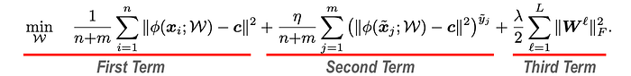
First term is for unlabeled data term, which minimizes the distance of unlabeled samples to the center c. It assumes most unlabeled data points are normal. The network tries to cluster these data points around c, making a compact normal class representation.

In practice, unlabeled datasets often include a few anomalies, which are typically rare and unidentified. However, the anomalies, due to their intrinsically different structure or features, tend to resist fitting into this tight cluster. They don’t minimize as easily as normal samples because their features are significantly different, causing them to remain somewhat distant from the center.

While the model tries to reduce distances, anomalies generally remain further away, becoming less tightly clustered. Anomalies often appear at the boundary regions or outskirts of the normal data cluster.

Once the training completes, latent space structure naturally reflects this dynamic:

A tight, dense cluster around c (mostly normal points).
Unlabeled anomalies generally remain further away, in peripheral regions, because they resisted full integration into the normal cluster.

Therefore, even if anomalies were unlabeled during training, the trained model can still detect them later based on distances in latent space.

The factor 1/(n+m) is a normalization term that computes the average loss per data point, considering all samples together (both labeled and unlabeled). Total number of samples = n+m. The sum terms are divided by n+m, ensuring the loss is scaled to an average.

By dividing by total samples, both labeled and unlabeled data contribute proportionally to the loss, creating balanced influence. Without this normalization, larger groups (e.g., unlabeled data) might dominate training disproportionately.

Second term is a labeled data term, which introduces explicit supervision from labeled samples.

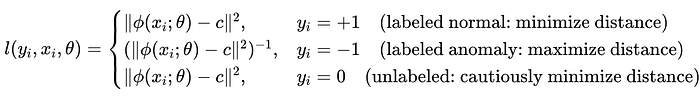
The multiplication by 𝑦̃ⱼ ensures labeled anomalies explicitly push away from the center c.

If 𝑦̃ⱼ = =+1 (normal sample), minimizes distance (pulls closer to c). Loss increases if distance is large and optimizer reduces distance.
If 𝑦̃ⱼ = = -1 (anomalous sample), maximizes distance (pushes away from c). Minimizing below expression is equivalent to maximizing the denominator ∥ϕ(xⱼ;W)−c∥². Thus, the optimization pushes anomalous points away from center c.

For anomalies (𝑦̃ⱼ = = -1 ), the term is:

To minimize the loss, the neural network has two choices:

Decrease numerator: Impossible, since numerator = 1 (fixed).
Increase denominator: The network increases the distance ∥ϕ(xⱼ;W)−c∥², pushing anomalies away.

Thus, anomalies are explicitly pushed outward.

If 𝑦̃ⱼ = = 0 (unlabeled sample), minimizes distance cautiously, gradually moves closer to the center. The training is careful not to overly assume all unlabeled points as normal, as there might be anomalies present.

Third term, is a standard weight decay regularization to prevent overfitting and ensure a smoother optimization landscape. It explicitly adds a cost to larger neural network weights.

Overfitting happens when a neural network learns training data too closely, including noise or irrelevant details, losing generalization to new, unseen data. B. Minimizing the third term pushes weights closer to zero, effectively shrinking their magnitude.

When we say we minimize the regularization term, we directly minimize the sum of squared weights:

Each individual weight Wℓ contributes positively (square) to this term. To minimize the sum of squares, the optimal solution is to make each term as close to zero as possible, because:

If the weight is large, say W = 10, the contribution to loss is 1⁰² = 100.
If the weight is small, say W = 0.1, the contribution is 0.¹²= 0.01, which is much smaller.

The minimum possible contribution from each weight is zero (⁰²=0), thus weights will naturally shrink toward zero.

Without regularization (λ=0) the weights can grow large and model tries excessively to minimize training error and the latent representations become overly specific to training set features including noise.

During neural network training, gradient descent updates the weights to minimize the total loss (including regularization):

The derivative of a single weight is:

Thus, the gradient update for regularization alone is proportional to the weight itself:

Here, α is the learning rate, and λ scales how strongly regularization affects the update. Each weight is directly subtracted by a small fraction proportional to itself. Large weights have larger corrections, shrinking them significantly. Small weights have tiny corrections, gently moving them closer to zero.

Effective on Unreliable Dataset

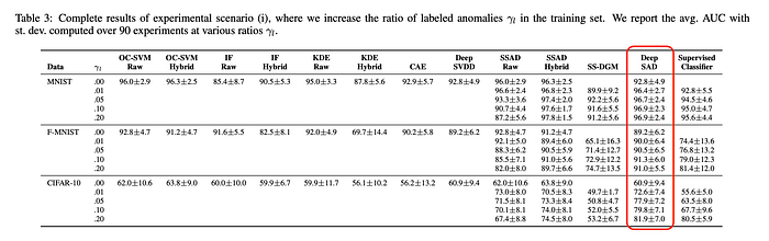
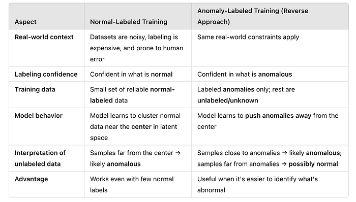
In real-world scenarios, datasets are often noisy, and labeling is both expensive and prone to human error. Even with a small amount of reliably labeled data, it’s possible to train models effectively for anomaly detection. The table below demonstrates how Deep SAD outperforms other methods as the proportion of labeled anomalies increases, highlighting its effectiveness in anomaly detection.

This approach can also be reversed with little bit of tweak: if we’re more confident about what constitutes an anomaly — but uncertain about what “normal” looks like — we can train the model using only labeled anomalies and treat the rest as unlabeled. During training, the model learns to push anomalies away from the center of the latent space. Samples that differ significantly from these anomalies can then be interpreted as normal, while unlabeled samples that fall close to the anomaly cluster are likely to be anomalous as well.